GPU Ray Tracer Using Ray Marching and Distance Fields

Introduction

In this article, we will be writing a simple ray tracer using the ray marching technique combined with distance field functions. If you are not familiar with the ray tracing technique, you should refer to the Wikipedia page.

This article was highly inspired by the work of Iñigo Quilez and his numerous resources on the subject (scroll all to the bottom for more!).

In order to make things more interactive and fun, we will be using WebGL once more and write the code directly within the fragment shader. That's right, it's a GPU-only ray tracer!

Note that for all the shader examples in this article, you can actually edit the GLSL code on the right and immediately see the result on the left (live WebGL preview).

(The live-editing currently does not tell you about compilation errors though, so make sure to double-check your code when nothing happens!)

Ray Marching with Distance Fields

Regular realtime rendering algorithms use heavy approximations to get a good tradeoff between drawing geometry fast and decent visuals.

Ray tracing on the other hand can be used to produce realistic scenes with a high level of details at the expense of more complex yet more accurate computations (simulate light ray physics).

A typical ray casting algorithm can be described as the following: for each 2D pixel in our output image (screen), we cast a ray of light directed towards the scene and evaluate geometry intersection(s) to compute the final pixel color.

In our implementation, the geometry in the scene is represented using distance fields function. These functions return the shortest distance between a given point and the surface of the geometry.

For instance, the distance to a sphere of radius r and centered in (0, 0, 0) can be represented as:

float sphere_dist(vec3 p, float r)
{
    return length(p) - r;
}

How do we simulate ray propagation?

A naive implementation would be to start from the origin position and progressively increment the position by a constant factor of the ray direction vector.

We can then compare each position against the distance methods to evaluate if we are intersecting with a scene element.

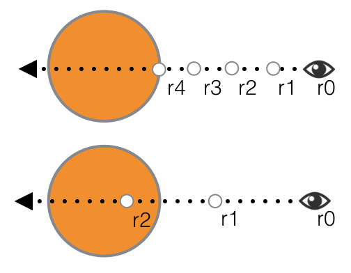
Raymarching with two different step values.
top: small step -> 4 iterations
bottom: larger step -> 2 iterations

Choosing a small step factor will result in precise collisions but also greatly increase the ray casting cost when trying to reach far distances.

On the other hand, a large factor speeds up the process but yield poor collision results making the overall quality worse...

Can we do better?

We can combine raymarching and distance field functions in order to step at a variable rate based on the scene geometry.

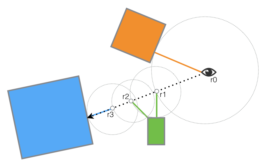
Ray Marching with Distance Field Functions

For a given ray position, we compute the distance to the closest element and move the ray that far. This distance is the maximum distance that the ray can cross without intersecting anything else.

We repeat this process and move the ray forward until:

• the closest distance is less than a very small epsilon value (intersection)
• the total step distance exceeds a threshold t_max (no intersection)
• the number of iterations is too high it_max (no intersection)

Render a Sphere

Ok this looks a bit funky, but it will help understand the basic implementation.

A good way to debug 3D rendering is to use... colors!

In the rendering above, we color each pixel using its corresponding (x, y, z) scene coordinates. Remember that colors are expressed in percent for each channel (red, green, blue). All the values are automatically clamped to [0, 1].

Time to dive into the code. Starting from the main() function.

void main()
{
    vec2 res = vec2(Resolution, 1.0);
    vec2 p = vec2(-1.0 + 2.0 * UV) * res;
    [...]
}

Quick reminder about the input variables:

• UV holds the current fragment coordinates (u, v) varying between [0.0, 1.0]
• Resolution is the ratio width / height of the viewport

The variable p holds the UV coordinates transformed from [0.0, 1.0] to [-1.0, 1.0]. p.x is scaled to the viewport ratio in order to avoid an horizontal stretching of the final rendering.

void main()
{
    [...]
    vec3 ro = vec3(0.0, 0.0, -2.0);
    vec3 rn = normalize(vec3(p, 1.0));
    [...]
}

We create a ray r with origin ro (camera position) and direction rn. Now notice that all the rays will be originating from ro but get a distinct direction based on the current fragment coordinates. Each of these rays put together cover a view frustum similar to the diagram below:

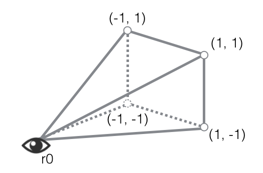
View Frustum

void main()
{
    [...]
    float t = ray_cast(ro, rn);
    vec3 pos = ro + t * rn;
    [...]
}

The parametric equation of a ray can be written as:

r(t) = ro + t * rn

If we consider that our ray moves over time (t in [0, +∞[), it will initially have the position r(0) = ro and may intersect with a scene element for some value t.

The method ray_cast(r0, rn) returns the smallest value of t for which we have a ray intersection.

Consequently, vec3 pos = ro + t * rn is the intersection location.

[...]

const float EPS = 0.002;  // precision 
const float T_MAX = 500.0;// max step value
const int IT_MAX = 50;    // max iterations

[...]

float ray_cast(vec3 ro, vec3 rn)
{
    float t = 0.0;
    for (int it = 0; it < IT_MAX; ++it)
    {
        vec3 pos = ro + t * rn; 
        float dt = sphere_dist(pos, 1.0);
        if (dt < EPS || t > T_MAX) {
            break;
        }
        t += dt;
    }
    return t;
}

Here we are! This is the meat of the raymarching algorithm as described in the diagram from the introduction.

Recall that the sphere_dist(pos, r) method returns the shortest distance between the position pos and the sphere centered in (0, 0, 0) of radius r=1.0.

Starting from t = 0.0, we advance the ray by dt = sphere_dist(pos, 1.0) and keep moving forward (t += dt) until:

• dt < EPS: The distance dt is almost zero, meaning that the sphere is super close (intersection).
• t > T_MAX: The total distance t is too big, we give up (no intersection)
• i >= IT_MAX: We iterated the process too many times, we give up (no intersection)

void main()
{
    [...]

    float t = ray_cast(ro, rn);
    vec3 pos = ro + t * rn;
    vec4 col = vec4(pos, 1.0);
    gl_FragColor = col;
}

Now back to the main() function. We have the scene coordinates of the ray intersection with the sphere.

In order to make sure that our computations are correct, we use the scene coordinates as debug colors for the final output pixel.

Background colors interpretation:

• Top-left: (-∞, +∞, +∞) -> (0.0, 1.0, 1.0)
• Bottom-left: (-∞, -∞, +∞) -> (0.0, 0.0, 1.0)
• Top-right: (+∞, +∞, +∞) -> (1.0, 1.0, 1.0)
• Bottom-right: (+∞, -∞, +∞) -> (1.0, 0.0, 1.0)

Sphere colors interpretation:

• Top-most pixel: (0.0, r, 0.0 -> (0.0, 1.0, 0.0)
• Right-most pixel: (r, 0.0, 0.0) -> (1.0, 0.0, 0.0)
• Top-right pixel: (r, r, 0.0) -> (1.0, 1.0, 0.0)
• Bottom-left area: (-r, -r, 0.0) -> (0.0, 0.0, 0.0)

Render a more complex scene

Below is a slightly more complex scene with:

• More than one element rendered at a time
• Different visuals (material) for each element

Let's review what got introduced in the code above!

void main()
{
    [...]
    vec2 result = ray_cast(ro, rn);
    float t = result.x;
    float material_id = result.y;
    [...]
}

The first thing to notice is that ray_cast(ro, rn) now returns a vec2 instead of a single float. This is nothing more than a trick to return more than one value from a function. Remember that t is the ray parameter for the closest visible point in the scene. If we want to render scene elements differently, we will need an extra bit of information to figure out which element did the ray hit, and that's exactly what material_id is used for.

In this scene, material_id = 0.0 means that we hit nothing (background) and all the integer values between 1.0 and 3.0 will tag one of the 3 scene elements.

// Modified ray_cast to handle the new material_id value.
vec2 ray_cast(vec3 ro, vec3 rn)
{
    float t = 0.0;
    float material_id = 0.0;
    for (int it = 0; it < IT_MAX; ++it)
    {
        vec3 pos = ro + t * rn; 
        vec2 result = ray_test(pos); 
        float dt = result.x;
        material_id = result.y;
        if (dt < EPS || t > T_MAX) {
            break;
        }
        t += dt;
    }
    if (t > T_MAX) material_id = 0.0;
    return vec2(t, material_id);
}

The raw_test(vec3 pos) method has been modified to handle more than one scene element:

vec2 ray_test(vec3 pos)
{
    vec2 d = min_dist(
        vec2(sphere_dist(pos, vec3(-1.0, 0.0, 0.0), 0.8), 1.0),
        vec2(sphere_dist(pos, vec3(1.0, 0.0, 0.0), 0.8), 2.0)
    );
    d = min_dist(d,
        vec2(sphere_dist(pos, vec3(0.0, 0.0, -0.5), 0.8), 3.0)
    );
    return d;
}

Notice that we evaluate the minimum distance for each scene element. This can obviously become very costly if the number of elements gets big!

The min_dist(vec2 r1, vec2 r2) is called using two tuples: ( t , material_id ) and will return the tuple with the lowest t value, meaning that once we evaluate all the distances, we get the closest element and its associated material id.

Now that we know how to get the material_id of a scene element, we can start doing some fancy lighting!

void main()
{
    [...]
    vec2 result = ray_cast(ro, rn);
    float t = result.x;
    float material_id = result.y;
    vec3 pos = ro + t * rn;

    vec4 col = vec4(0.0, 0.0, 0.0, 1.0);

    if (material_id > 0.0) {
        vec3 n = compute_normal(pos); 
        float diffuse = dot(n, -rn); 
        vec3 ambient; 
        if (material_id == 1.0) {
            ambient = vec3(1.0, 0.5, 0.5); 
        }
        else if (material_id == 2.0) {
            ambient = vec3(0.5, 0.5, 1.0); 
        }
        else {
            ambient = vec3(0.5, 1.0, 0.5);
        }
        col = vec4(ambient * diffuse, 1.0);
    }

    gl_FragColor = col;
}

Our lighting equation is super simple:

col = vec4(ambient * diffuse, 1.0);

• vec3 ambient is the color of the element (we assume it is uniformly of the same color).
• float diffuse is the dot product between the opposite of the ray direction and the normal of the surface we hit.

By definition of the dot product:

dot( a , b ) = ||a|| * ||b|| * cos( theta ).

theta being the angle between the two vectors.

Since the two vectors are normalized, we can simplify to:

dot( a , b ) = cos( theta )

Consequently:

• If the ray is going in the same direction as the surface normal, we get a bright pixel: cos(theta) -> 1.0.
• If the ray is perpendicular to the surface normal, we will get a darker color: cos(theta) -> 0.0.

BONUS:

The method vec3 compute_normal(vec3 pos) takes as an input the position at which the ray hit some surface and returns the normal of that surface.

const float EPS = 0.002;  // precision 
vec3 compute_normal(vec3 pos)
{
    vec3 eps = vec3(EPS, 0.0, 0.0);
    vec3 n = vec3(
        ray_test(pos+eps.xyy).x - ray_test(pos-eps.xyy).x,
        ray_test(pos+eps.yxy).x - ray_test(pos-eps.yxy).x,
        ray_test(pos+eps.yyx).x - ray_test(pos-eps.yyx).x );
    return normalize(n);
}

For each dimension of the vector n, we cast two rays at positions slightly off in one dimension from the original position.

// Move slightly on the x dimension.
vec3 p1 = pos + eps.xyy;
vec3 p2 = pos - eps.xyy;

If the surface is flat in the dimension we are exploring, then the difference of the two t values will be 0. On the other hand, if there is an offset, that means that our normal needs to expand in that direction.

Let's simplify by dropping one dimension and try to visualize what is going on:

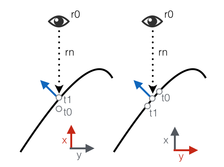
compute_normal in two dimensions.

On the left, x axis:

• t0 goes below the original t value (since ray_test returns the shortest distance, we return t0).
• t1 will converge to the original t value.

On the right, y axis:

• t0 goes above the original t value since the surface is hit higher.
• t1 goes below the original t value since the surface is hit lower.

These two offsets combined together represent a good approximation of the 2D surface normal (after normalization of course).

Learn More

Now it's time to start experimenting! You can find all sort of crazy examples on shadertoy.

If you want to learn more about ray marching and distance field functions, I strongly recommend Iñigo Quilez's website:

• Distance Functions
• Shadows for Raymarching Distance Fields
• Terrain Marching